
The faster things run, the more we can do.
For AG Studio, that means a snappier UI or more data per query. We want both, in a dashboard that runs entirely in the browser.
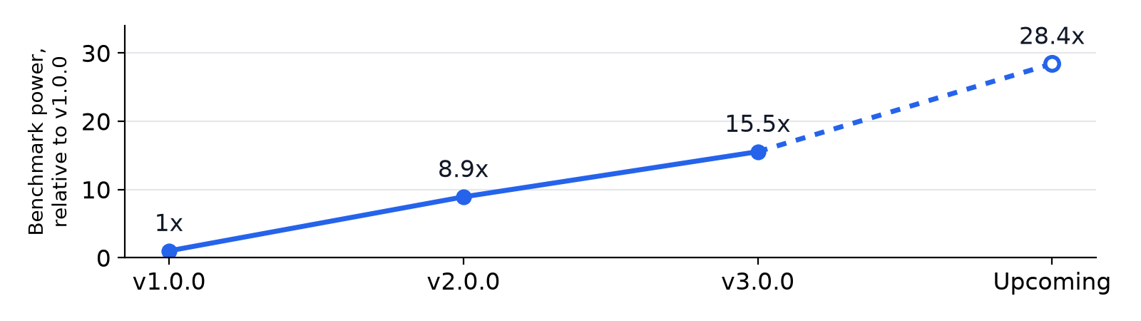
The chart above tracks the engine's progress since the v1.0.0 release, using our internal benchmark suite.
I look after AG Studio's data engine. In this post, I'll cover two areas where I've made it faster, and how that helps developers and their users get more out of it.
Why I wrote AG Studio's built-in data engine
AG Studio runs inside other people's applications. The developers who embed it often don't control where those applications are deployed, and some deploy into locked-down environments. Their compliance teams may also limit which dependencies they can add. That's why AG Studio, like all our products, has zero external dependencies. It's also why I wrote AG Studio's own data engine rather than build on an open source in-browser database.
The engine has to work within whatever limits each deployment sets. Some deployments block Web Workers, WebAssembly or new Function through their Content Security Policy. Others don't send the COOP/COEP headers that SharedArrayBuffer needs. I take the most restrictive policy as my baseline. If the engine runs there, it runs anywhere.
AG Studio is an interactive business intelligence (BI) component. It manages widgets, their configuration and the data they display, so a lot happens before a query reaches the engine. Studio batches widget queries, applies cross-filtering and highlighting, plans and optimises each query, resolves joins, handles pre- and post-aggregation, and splits expressions by locality. Then it hands the batch to the data engine.
Developers can connect data in three ways:
- a plain local array
- an
async getData()call they write themselves, to fetch JSON or API data on demand - their own engine in place of ours, running locally in the browser or talking to a remote server
The built-in engine follows the HOLAP (hybrid OLAP) model, which works over both pre-computed summaries and detail rows. The difference is that the engine computes those summaries, or cubes, on demand rather than ahead of time. Pre-computing every combination a user might slice by would cost memory and load time that a browser tab can't spare.
Without Web Workers, all of the engine's work runs on the browser's main thread, where it competes with the UI for processing time. The engine yields to the page between chunks of work so that a long query doesn't freeze it. Memory allocation and garbage collection run on the same thread too. That's three things competing for the same time, and users see the contention as page freezes or stuttering interactions.
That left me two options:
- do less work on the main thread
- create less garbage for the collector
Where optimisation work happens
Across the whole engine, I sort optimisation work into five buckets:
- Algorithmic: a better technique for the same problem, such as join build-side selection or dictionary encoding.
- Process: how work is scheduled and batched across a session.
- Query: what the planner decides before execution starts.
- Memory: how much memory a query uses, how often it allocates, and what reclaiming it costs.
- V8: code shaped for the JavaScript engine the rest runs on.
Within query planning, some of the more interesting steps are:
- Logical query optimisation
- Predicate/Sort/Window pushdown
- Expression splitting
- Join type selection
- Multi-join path selection
- Physical query optimisation (built-in engine)
- Column storage
- Operation sequencing
- Operation fusion
- Join implementations, including cardinality-driven build-side selection
- Caching
- Chunking
This post picks one example for each option, both chosen because our users hit them constantly: query optimisation (cross-filters) to do less work, and memory optimisation (arenas and pools) to create less garbage.
Making cross-filters do less work
Cross-filtering is the bread and butter of interactive BI tools, and that drives my never-ending push to make it as fast as possible.
A cross-filter narrows the rest of a dashboard to the user's selection. Take a dashboard with two widgets: revenue by month, and top products. Click March on the first, and Studio adds a condition, month = March, to the query behind every other widget, then reruns them.
The top-products widget reads from two tables. Its product and quantity columns come from order items, but the order date lives on orders. To apply the March filter, the query has to join order items to orders, work out each order's month from its date, and then keep only the March rows.
A filter is cheapest at the start of a query, before any join, so that everything after it handles one month of rows instead of all of them. Moving filters down towards the table scans is called predicate pushdown, and the planner already does it. For a filter on a stored column, such as a region, that works. A month filter got stuck. I’d left two gaps in the planner that kept it above the join. The left side of the diagram shows the old plan, and the numbers on the right show where each fix changes it.
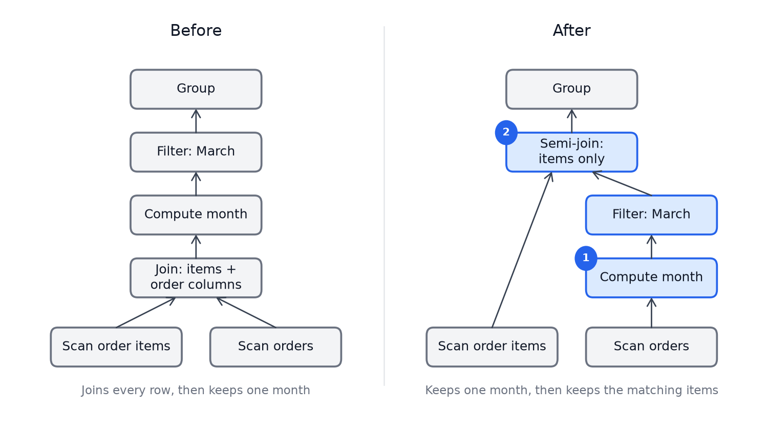
1. Month isn't a stored column. The engine computes it from the order date, and the planner used to place that computation above the join, so the filter had to wait there too. Now, when a filter depends on a computed field, the planner moves the computation below the join and the filter follows it down. Without such a filter, the planner leaves the computation where it is: below the join it might run over more rows or fewer, and the planner has no row counts to decide with.
That's a deliberate behaviour. I'd rather the planner only make changes it can prove help than ones it has to guess at. Not every data source can supply row counts, and a planner that relied on them would plan the same query differently depending on where its data came from.
My first version of this never fired on a real query. Two bugs hid it. One step rebuilt every join clause and silently dropped the flag marking it as filter-only. Another step often picks the date table to start the join chain, and the starting table never gets a join clause of its own, so it could never be marked at all. I now check changes like this against the real execution with EXPLAIN ANALYZE, not just the plan.
Getting it right cut the benchmark's cross-filter pass by 58%.
2. When a query joined a table only because a filter referred to it, and each row matched at most one row in that table, Studio used to give it an ordinary join. Order items joined to orders for a March filter are one example: each item belongs to one order. An ordinary join carries the orders' columns into the result, even though nothing reads them. Studio now uses a semi-join, which keeps the matching items and adds no columns. This cut the same pass by 19%.
Pushdown has limits, though. A filter can only move below a join if everything it needs comes from one side of that join. A condition that compares fields from both tables, such as items shipped more than a week after their order date, has to wait until the join has brought those fields together. The same goes for a filter on an aggregated value, such as products with more than 1,000 sales in total: the total doesn't exist until the grouping has run. And a filter on the optional side of an outer join can't move below it without changing which rows come back. In each case, the planner keeps the filter where the result stays correct, even if that's later than I’d like.
Silent failures worry me more than crashes: a crash gets reported. An optimisation that quietly never runs just looks like a slow feature. An optimisation that gives incorrect results may pass unseen. Where the engine depends on an assumption holding, I'd rather it throw than carry on with a corrupted state.
I never trade correctness for speed. The bugs that worry me most are the ones that type-check, pass every unit test and still return the wrong number. So before I look at a change's timings, it has to reproduce the same result hashes on every benchmark query, and every fix comes with a test I've watched fail without it.
Both fixes follow the same rule: apply the filter as early as the query allows, and don't carry anything through the plan that the result doesn't need. Studio chooses the semi-join itself, before the query reaches an engine, so custom engines get it too. The built-in engine's planner handles the month calculation. Either way, a month cross-filter now shrinks the data before the expensive part of the query rather than after it.
Arenas and pools
A query that creates thousands of small typed arrays hands the garbage collector thousands of buffers to track and release. Each one brings the next collection closer, and on the main thread a collection means a stutter.
I don't control the garbage collector, but I can control some of what triggers it. The engine uses a family of manually controlled memory structures, including arenas and pools. They reduce garbage collection during queries and let me guide when the eventual collection happens.
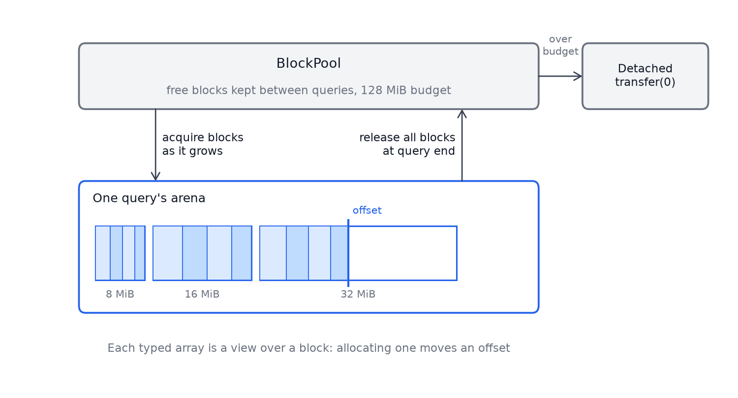
An arena is one large pre-allocated buffer that the engine carves into smaller pieces itself. The biggest distinction for me between arenas and pools is their lifecycle: the engine releases an arena all at once when the query ends, whereas a pool keeps buffers to hand out again.
The engine uses two pools. BlockPool supplies the large blocks that arenas and cache entries are built from. A separate typed-array pool recycles the small arrays that individual operations use.
Concretely, the engine's arenas hand out typed-array views over one large buffer:
allocateFloat64(count: number): Float64Array {
    const byteOffset = align(this.offset, 8);
    this.offset = byteOffset + count * 8;
    return new Float64Array(this.buffer, byteOffset, count);
}
Allocating just moves an offset, which is why it's cheap. The engine never frees a single allocation. It releases the whole arena when the query ends. To let an arena grow, ChainedArena adds a block when a computation outgrows the current one, each twice the size of the last, up to a cap. Doubling keeps the block count low for big queries without wasting memory on small ones.
A full query batch with about 300 MiB of intermediate data uses about ten blocks. The blocks come from BlockPool, which keeps up to 128 MiB of released blocks for the next query. I’ve tuned these values to common workloads.
When a result goes into a cache, the engine copies its columns and join indices into one buffer, taken from BlockPool and kept for as long as the entry. The collector then sees one buffer per cache entry, not one per column, at the cost of copying the data once.
Joins follow the same pattern. A join sizes its hash table up front, so it never has to grow it and throw away the old arrays mid-build. It builds the table in one arena and takes that arena's buffer from BlockPool.
When a released block would take the pool over its budget, the engine detaches it with block.transfer(0), so its memory can be released right away instead of waiting for the collector.
Keeping blocks between queries pays off when queries run back to back, as they do on a dashboard. To measure it, I ran the dashboard benchmark with BlockPool reuse switched off, alternating five runs of each, so that drift in the machine or the JIT affected both sides equally.
Reusing blocks saved 11% of the time for a dashboard render followed by a cross-filter, and 25% of its time in garbage collection. The cross-filter pass on its own spent 53% less time collecting garbage.
Pooling doesn't always help. I tried pooling the arrays a scan creates for each column, and garbage collection got worse: pause time rose by 82%, the number of collections by 60%, and collection overhead went from 9.4% to 17% of total time. The longest pause more than tripled, from 102 to 329 ms. Those arrays live as long as the cached data, and the pool holds on to them long enough for the collector to move them into its older generation, where collections are slower. So they stay out of the pool.
Freeing memory by hand reintroduces the risk of use-after-free, since a reload can replace data while a query is still reading it. Each query therefore pins the generation of cached data it started with, and a reload's cleanup waits until the last query using the old generation finishes.
Managing memory manually adds work and risk. For a dashboard that runs queries back to back on the main thread, the numbers show it pays off.
Wrapping up
Both changes in this post go back to the two options I started with. Moving the month filter below the joins means the engine does less work on the main thread. Arenas and pools mean it leaves less garbage for the collector.
Neither change is a breakthrough on its own. The chart at the top of this post is the sum of many changes like these. I measure every change, and sometimes the numbers tell me not to do something, as they did when I tested pooling for column storage.
I do most of my profiling in V8, because Node and d8 make it easy. But I also measure in JavaScriptCore and SpiderMonkey, so the gains reach Safari and Firefox users as well as Chrome users.
Measuring is harder than it sounds. Early on, my own GC analyser reported that garbage collection took 65.7% of a benchmark run. The real figure was 5.5%: the tool had merged timestamps from separate processes, each with its own clock starting near zero. Now I check the measuring tools as carefully as the engine.
Micro-benchmarks can mislead too. My per-operator expression benchmarks each isolated one operator, so an expression the fast path couldn't handle at all scored just as well as one it covered completely. I now measure end to end over real data, and from a cold start by default, because that's what a user's first query sees. And the numbers we’re looking at are per-operator, or per query. How the overall engine speeds up from individual changes is more nuanced.
The "Upcoming" point on the chart is coming soon. In future posts I'll cover other areas I skipped here, including how the engine schedules and batches work across a session, and how I shape code for the JavaScript engines it runs on.